TimescaleDB Compression: A Complete Guide to 95%+ Storage Reduction

TimescaleDB Compression: A Complete Guide to 95%+ Storage Reduction

Time-series data grows fast. An IoT fleet of 1,000 sensors reporting every 10 seconds generates 8.6 million rows per day — roughly 500 MB of raw PostgreSQL heap data. After a month, you're looking at 15 GB. After a year, 180 GB. TimescaleDB's native columnstore compression can reduce that by 10–20x, turning 180 GB into 9–18 GB.

This guide covers how TimescaleDB compression actually works, how to configure it properly, and what results to expect with real data.

How Columnstore Compression Works

TimescaleDB compression converts row-oriented PostgreSQL heap tables into a column-oriented format. Instead of storing complete rows sequentially, it groups values by column and applies type-aware encoding:

• Delta-of-delta for timestamps: Regular intervals (e.g., every 10 seconds) compress to near-zero storage because only the deviation from the expected pattern is stored.
• Gorilla encoding for floats: Consecutive sensor readings that differ by small amounts (e.g., temperature fluctuating between 20.1°C and 20.3°C) encode in just a few bits per value.
• Dictionary encoding for low-cardinality integers and text: Repeated values like status codes or device types store a lookup table plus small indexes.
• LZ compression for high-entropy data: Applied as a final pass on top of the type-specific encoding.

The result is that typical IoT sensor data — regular timestamps, slowly-changing floats, repeated categorical values — compresses dramatically.

Configuring Compression: segmentby and orderby

Compression configuration requires two decisions: segmentby and orderby.

segmentby — How Data Is Grouped

The segmentby column determines how rows are grouped into compressed segments. Each unique value creates a separate segment within a chunk. This matters because:

• Queries that filter on the segmentby column only decompress the relevant segments
• The column should have moderate cardinality — 100 to 10,000 unique values per chunk is ideal

-- Enable compression with device_id as segment column
ALTER TABLE sensor_readings SET (
    timescaledb.compress,
    timescaledb.compress_segmentby = 'device_id',
    timescaledb.compress_orderby = 'reading_timestamp DESC'
);

For an IoT table with 1,000 devices and 1-day chunks containing 8.6M rows, each segment holds ~8,600 rows — enough data for the column encoders to find patterns and compress effectively.

orderby — How Data Is Sorted Within Segments

The orderby column controls the physical sort order within each segment. Almost always, this should be your time column in descending order. This enables:

• Efficient range scans on recent data (most common query pattern)
• Better delta encoding on the timestamp column itself
• Implicit ordering that eliminates explicit ORDER BY in queries

Adding a Compression Policy

After configuring compression settings, add an automated policy:

-- Compress chunks older than 1 hour automatically
SELECT add_compression_policy('sensor_readings',
    compress_after => INTERVAL '1 hour');

The compress_after interval determines how long a chunk stays uncompressed (in row format) before the background worker compresses it. A shorter interval saves more space but means recent data is compressed sooner, which adds a small decompression overhead for queries hitting that time range.

For most workloads, compress_after => INTERVAL '1 hour' is a good starting point. High-frequency query patterns on recent data might benefit from '4 hours' or '1 day'.

Real-World Compression Results

Running against a test dataset of 1 million IoT sensor readings (temperature, humidity, pressure, battery voltage, signal strength) across 100 devices with 1-day chunks:

| Metric | Value | |--------|-------| | Before compression | ~120 MB | | After compression | ~8 MB | | Compression ratio | 15x | | Space reduction | 93% |

The float columns (temperature, humidity, pressure) compress best because gorilla encoding exploits their slow-changing nature. The timestamp column compresses to near-zero due to its regular 1-minute intervals.

Query Performance on Compressed Data

A common concern is that compression hurts query performance. In practice, compressed data often queries faster than uncompressed data for analytical workloads:

-- This query benefits from columnar scan
EXPLAIN ANALYZE
SELECT device_id, AVG(temperature), COUNT(*)
FROM sensor_readings
WHERE reading_timestamp >= now() - INTERVAL '7 days'
GROUP BY device_id;

TimescaleDB's ColumnarScan operator reads only the columns needed by the query, skipping irrelevant columns entirely. For a SELECT AVG(temperature) on a table with 7 columns, the engine reads ~14% of the data compared to a full heap scan.

Point queries filtered on segmentby decompress only the matching segment. A query for device_id = 42 over the last day touches one segment (~8,600 rows) instead of the entire chunk (~8.6M rows).

How myDBA.dev Monitors Compression Health

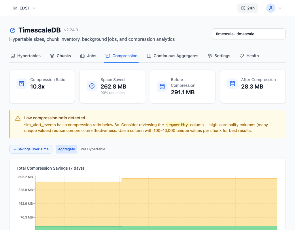
The TimescaleDB monitoring page in myDBA.dev provides continuous visibility into compression effectiveness. The Compression tab shows per-hypertable compression ratios, before/after sizes, and segmentby/orderby configuration at a glance. When a hypertable's ratio drops below 3x, a recommendation panel flags it with specific guidance on reviewing the segmentby column's cardinality.

The Chunks tab visualizes the compression timeline — green bars for compressed chunks, orange for uncompressed — making it easy to spot gaps where compression has fallen behind.

Common Pitfalls

1. Inserting into compressed chunks. TimescaleDB supports DML on compressed data, but each INSERT/UPDATE/DELETE must decompress the affected segment, modify it, and recompress. Batch operations work, but high-frequency single-row inserts into compressed chunks are slow. Keep the active (most recent) chunk uncompressed via compress_after.

2. Schema changes. Adding or removing columns on a table with compressed chunks requires decompressing first. Plan schema changes during maintenance windows.

3. No compression policy. Enabling compression settings (ALTER TABLE ... SET) without adding add_compression_policy() means nothing gets compressed automatically. The settings just declare how to compress — the policy triggers when.

Preventing Storage Bloat

Enable compression on every hypertable that stores time-series data. The overhead is minimal, and the space savings compound over time. Pair compression with a retention policy (add_retention_policy) to automatically drop chunks beyond your retention window — compressed chunk drops are instant with no decompression required.

Monitor compression ratios continuously. A sudden drop in ratio often signals a schema change, a new high-cardinality column, or a misconfigured segmentby. Tools like myDBA.dev surface these issues through health checks (T5 for low compression ratio, T9 for uncompressed chunk percentage) before they consume significant storage.

The combination of compression + retention + monitoring turns TimescaleDB storage management from a manual chore into an automated pipeline.