How TimescaleDB Chunks Actually Work (And Why Size Matters)

How TimescaleDB Chunks Actually Work (And Why Size Matters)

TimescaleDB's hypertable abstraction makes it easy to forget that your data lives in hundreds — sometimes thousands — of ordinary PostgreSQL tables. These underlying tables are called chunks, and their size, count, and configuration have a direct impact on query planning time, compression efficiency, and retention granularity. Understanding how chunks work is the difference between a TimescaleDB deployment that scales and one that grinds to a halt at a few hundred gigabytes.

What Chunks Actually Are

When you call create_hypertable(), TimescaleDB converts a regular PostgreSQL table into a hypertable — a virtual table that automatically partitions incoming rows across many physical tables called chunks. Each chunk covers a specific time interval and is implemented as a real PostgreSQL table in the _timescaledb_internal schema.

-- Create a hypertable with 1-day chunks
SELECT create_hypertable('sensor_readings', 'recorded_at',
    chunk_time_interval => INTERVAL '1 day');

Each chunk gets a CHECK constraint that bounds its time range:

-- Internal chunk constraint (auto-generated)
-- CHECK (recorded_at >= '2026-02-01 00:00:00' AND recorded_at < '2026-02-02 00:00:00')

These constraints are the mechanism that makes time-based queries fast. When you insert a row, TimescaleDB routes it to the correct chunk based on the timestamp. When you query, PostgreSQL uses these constraints to skip irrelevant chunks entirely.

How Constraint Exclusion Works

PostgreSQL's query planner evaluates each chunk's CHECK constraint against your WHERE clause before executing the query. If the constraint proves a chunk cannot contain matching rows, the planner excludes it entirely — no I/O, no buffer reads, no index lookups on that chunk. This is called constraint exclusion, and it's the core mechanism that makes TimescaleDB competitive with purpose-built time-series databases.

EXPLAIN ANALYZE
SELECT * FROM sensor_readings
WHERE recorded_at >= '2026-02-20' AND recorded_at < '2026-02-21';

In the EXPLAIN output, you'll see a line like:

Chunks excluded during startup: 347

This means 347 chunks were evaluated and skipped because their time constraints didn't overlap with the query's time range. Only the matching chunks (in this case, one chunk for February 20th) are actually scanned.

The critical detail: without a time predicate in your WHERE clause, PostgreSQL cannot exclude any chunks. A query like SELECT COUNT(*) FROM sensor_readings WHERE device_id = 42 — with no timestamp filter — must open and scan every chunk in the hypertable. This is the most common performance mistake with TimescaleDB: filtering on non-time columns without bounding the time range. Even if device_id is indexed, the planner generates an append plan across all chunks, creating one index scan node per chunk. Adding AND recorded_at >= now() - INTERVAL '7 days' narrows the scan to a handful of chunks and transforms query performance.

Why Chunk Count Matters

Even though excluded chunks aren't scanned, the planner still evaluates every chunk's constraint during planning. This evaluation has a cost that scales linearly with chunk count.

The impact is measurable. In a controlled test against the same dataset, the planning overhead was dramatic:

| Chunk Count | Planning Time | Execution Time | Total Time | |-------------|---------------|----------------|------------| | 4,322 chunks (1-hour interval) | 443 ms | 2 ms | 445 ms | | 26 chunks (7-day interval) | ~5 ms | 2 ms | 7 ms |

The query was identical — a simple time-bounded SELECT hitting a single day's data. Execution time was the same because the same rows were scanned. But the planner spent 443 ms just evaluating and excluding 4,321 irrelevant chunks.

-- Same query, vastly different planning times based on chunk count
EXPLAIN ANALYZE
SELECT AVG(temperature)
FROM sensor_readings
WHERE recorded_at >= '2026-02-20' AND recorded_at < '2026-02-21';

-- With 4322 chunks:  Planning Time: 443.201 ms  Execution Time: 2.105 ms
-- With 26 chunks:    Planning Time: 4.892 ms    Execution Time: 2.098 ms

At 3,000+ chunks, you're adding hundreds of milliseconds to every query — even trivial ones. This overhead compounds in dashboards that issue 10-20 parallel queries, turning a 50 ms page load into a 5-second wait. The overhead also affects prepared statements: each PREPARE re-evaluates constraints, so connection pools that reprepare on checkout pay the planning cost repeatedly. This is why chunk count is often the first thing to check when TimescaleDB queries feel slow despite adequate indexing.

Choosing the Right Chunk Interval

The goal is to keep total chunk count manageable while maintaining chunks large enough for efficient compression. TimescaleDB recommends targeting approximately 25 million rows per chunk as a starting point.

The formula:

chunk_interval_seconds = target_rows_per_chunk / rows_per_second

For a sensor fleet ingesting 100 rows per second:

25,000,000 / 100 = 250,000 seconds ≈ 2.9 days

A 3-day chunk interval would keep each chunk around 25M rows. For higher ingest rates (1,000 rows/second), a 7-hour interval produces similar chunk sizes.

To change the interval on an existing hypertable:

-- Change chunk interval for future chunks (existing chunks are unaffected)
SELECT set_chunk_time_interval('sensor_readings', INTERVAL '3 days');

The key limitation: set_chunk_time_interval() only affects chunks created after the change. Existing chunks retain their original interval. This means that after a change, you'll have a mix of old-interval and new-interval chunks until the old ones age out of your retention window.

To verify your current chunk count and sizes:

-- Check chunk count and average size per hypertable
SELECT
    hypertable_name,
    count(*) AS total_chunk_count,
    pg_size_pretty(avg(total_bytes)) AS average_chunk_size
FROM timescaledb_information.chunks
GROUP BY hypertable_name
ORDER BY total_chunk_count DESC;

Monitoring Chunk Health with myDBA.dev

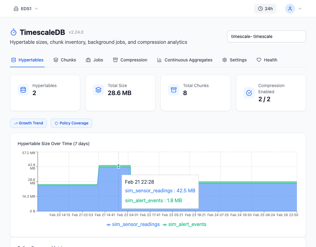
Chunk proliferation is a gradual problem — it doesn't trigger errors until planning overhead becomes noticeable. myDBA.dev's TimescaleDB health checks catch this early. Health Check T2 warns when a hypertable's chunk count exceeds safe thresholds, flagging tables before they cross the 1,000-chunk boundary where planning overhead starts to bite.

The Chunks tab provides a timeline visualization of every chunk — its time range, compression status, and size — making it straightforward to spot interval misconfigurations or retention gaps.

Prevention Checklist

Set the interval based on your ingest rate. Calculate expected rows per chunk using the formula above. Aim for 25M rows per chunk as a baseline, adjusting for your query patterns.

Use retention policies to cap chunk count. The add_retention_policy() function automatically drops chunks older than your retention window:

-- Automatically drop chunks older than 30 days
SELECT add_retention_policy('sensor_readings', drop_after => INTERVAL '30 days');

Dropping a chunk is an instant metadata operation — PostgreSQL removes the underlying table file rather than deleting rows individually. There is no dead tuple accumulation, no vacuum overhead, and no transaction ID consumption. This keeps your total chunk count bounded regardless of ingest rate, and it's one of the key advantages of the chunk-based architecture over plain partitioning with manual DELETE statements.

Monitor chunk count trends. A rising chunk count with a stable ingest rate means your interval is too small. myDBA.dev's Hypertables tab tracks chunk counts over time, making trend shifts visible before they reach the performance threshold.

The chunk is the fundamental unit of TimescaleDB's performance model. Get the interval right, keep the count bounded, and most TimescaleDB performance problems never materialize.