Optimizing Continuous Aggregate Performance for Large Datasets

Optimizing Continuous Aggregate Performance for Large Datasets

Your continuous aggregate refresh job used to take two seconds. Now it takes 30 minutes, the materialization hypertable is eating 40 GB of disk, and the refresh is blocking one of your limited background worker slots for the entire duration. This is the predictable outcome of a common setup mistake: choosing a bucket size based on query convenience without considering what it does to the materialization table underneath.

Continuous aggregates (CAGGs) are one of TimescaleDB's most powerful features — they pre-compute aggregations incrementally so your dashboards read from a compact summary instead of scanning raw data. But the materialization hypertable that backs a CAGG is a real hypertable with real chunks, real indexes, and real storage costs. Treat it carelessly and it becomes the performance problem it was supposed to solve.

Bucket Size Is the Biggest Lever

The single most impactful decision when creating a CAGG is the bucket width. It determines how many rows end up in the materialization table, which in turn controls refresh duration, disk usage, and query speed against the aggregate.

Consider a source hypertable with 10 million rows over 30 days, collected from 200 devices. Here is what happens when you materialize the same data at three different bucket widths:

| Bucket Size | Materialized Rows | Materialization Size | Refresh Duration (full) | |-------------|-------------------|----------------------|------------------------| | 1 minute | ~8.6 million | ~500 MB | 30-60 seconds | | 1 hour | ~144,000 | ~15 MB | 5-10 seconds | | 1 day | ~6,000 | ~1 MB | < 1 second |

The 1-minute CAGG materializes nearly as many rows as the source table. You have pre-computed averages and counts, but the materialization itself is a large hypertable that needs its own compression, its own retention policy, and its own index maintenance. The 1-hour CAGG reduces the row count by 60x and the size by 30x. The 1-day CAGG is trivially small.

-- 1-hour buckets: the sweet spot for most dashboards
CREATE MATERIALIZED VIEW metrics_hourly
WITH (timescaledb.continuous) AS
SELECT
    time_bucket('1 hour', event_timestamp_utc) AS bucket_utc,
    device_id,
    AVG(metric_a) AS avg_metric_a,
    MAX(metric_b) AS max_metric_b,
    COUNT(*) AS event_count
FROM raw_device_metrics
GROUP BY bucket_utc, device_id;

The rule of thumb: your bucket width should match the resolution your queries actually need. If your dashboard plots hourly data points, a 1-minute CAGG is doing 60x more work than necessary during every refresh cycle.

Refresh Window Tuning

The default refresh policy recomputes the entire CAGG on every run. For a large dataset, this is catastrophically wasteful. The add_continuous_aggregate_policy() function accepts three parameters that bound the refresh window:

SELECT add_continuous_aggregate_policy('metrics_hourly',
    start_offset  => INTERVAL '3 hours',  -- only re-aggregate last 3 hours
    end_offset    => INTERVAL '1 hour',   -- skip the most recent incomplete bucket
    schedule_interval => INTERVAL '1 hour'
);

start_offset controls how far back the refresh looks for changed data. Set this to cover the maximum latency of late-arriving rows plus one extra bucket width as a safety margin. If your data arrives within 30 minutes of its timestamp, a 2-hour start_offset with 1-hour buckets gives comfortable headroom.

end_offset defines how close to "now" the refresh will materialize. Setting this to at least one bucket width avoids materializing partial buckets that will be immediately invalidated on the next refresh. For a 1-hour CAGG, use INTERVAL '1 hour'.

schedule_interval should be less than or equal to start_offset. If your refresh runs every hour but only looks back 30 minutes, you will miss data that arrived in the gap.

A tightly tuned refresh window means the job processes a few hours of data instead of 30 days. The refresh duration drops from minutes to milliseconds, and the background worker slot is freed almost instantly.

Compress the Materialization Table

The materialization hypertable is a regular hypertable, which means it supports compression. This is often overlooked because the CAGG abstraction hides the underlying table, but the savings are substantial — typically 10-20x size reduction on the materialization data.

-- Find the materialization hypertable name
SELECT materialization_hypertable_schema || '.' || materialization_hypertable_name
FROM timescaledb_information.continuous_aggregates
WHERE view_name = 'metrics_hourly';
-- Returns something like: _timescaledb_internal._materialized_hypertable_42

-- Enable compression on the materialization hypertable
ALTER TABLE _timescaledb_internal._materialized_hypertable_42 SET (
    timescaledb.compress,
    timescaledb.compress_segmentby = 'device_id',
    timescaledb.compress_orderby = 'bucket_utc DESC'
);

-- Add a compression policy (compress chunks older than 1 day)
SELECT add_compression_policy(
    '_timescaledb_internal._materialized_hypertable_42',
    compress_after => INTERVAL '1 day'
);

The segmentby column should match your most common filter column in queries against the CAGG. If you typically filter by device_id, segment by device_id. The orderby column should be the bucket column in descending order, since most dashboard queries fetch the most recent data first.

Indexing the CAGG

TimescaleDB creates a default index on the bucket column, but queries against the CAGG often filter by additional dimensions. If your dashboards always filter by device_id, add a composite index:

CREATE INDEX ON metrics_hourly (device_id, bucket_utc DESC);

This index serves range queries like "show me device 42's last 7 days" without scanning the full materialization. Without it, every query against the CAGG performs a sequential scan filtered by the bucket index alone, then applies a recheck on device_id.

Hierarchical CAGGs for Multi-Resolution

Rather than creating one CAGG and hoping the bucket size works for every use case, build a hierarchy. A fine-grained CAGG feeds into a coarser one:

-- Level 1: hourly summary from raw data
CREATE MATERIALIZED VIEW metrics_hourly
WITH (timescaledb.continuous) AS
SELECT time_bucket('1 hour', event_timestamp_utc) AS bucket_utc,
       device_id, AVG(metric_a) AS avg_metric_a, COUNT(*) AS event_count
FROM raw_device_metrics
GROUP BY bucket_utc, device_id;

-- Level 2: daily summary from the hourly CAGG
CREATE MATERIALIZED VIEW metrics_daily
WITH (timescaledb.continuous) AS
SELECT time_bucket('1 day', bucket_utc) AS bucket_utc,
       device_id, AVG(avg_metric_a) AS avg_metric_a, SUM(event_count) AS event_count
FROM metrics_hourly
GROUP BY bucket_utc, device_id;

Each tier can have its own refresh policy, retention policy, and compression settings. The daily CAGG refreshes from the already-compact hourly materialization instead of rescanning 10 million raw rows. Your real-time dashboard queries the hourly CAGG. Your monthly reporting queries the daily one. Neither is doing unnecessary work.

How myDBA.dev Helps

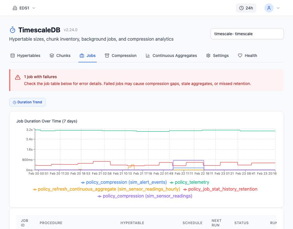
myDBA.dev's Jobs tab tracks every CAGG refresh execution, plotting duration trends over time. A refresh that crept from 2 seconds to 45 seconds over the past month is immediately visible as an upward trend line, letting you catch bucket sizing problems before they consume your background worker budget.

Sizing Guidelines

Match bucket width to query resolution. If your finest dashboard granularity is hourly, use 1-hour buckets. Minute-level buckets should be reserved for real-time alerting use cases where sub-minute latency matters.

Compress the materialization hypertable. It is a real hypertable. Treat it like one. Segment by your primary filter dimension, order by the bucket column descending, and set a compression policy.

Use hierarchical CAGGs for multi-resolution access. An hourly CAGG for recent data and a daily CAGG for historical queries gives you both granularity and compactness without materializing everything at the finest resolution.

Tighten the refresh window. A start_offset of 2-3x your bucket width covers late-arriving data without reprocessing the entire dataset. Set end_offset to at least one bucket width to avoid partial-bucket churn.

The materialization table behind a continuous aggregate follows the same performance rules as any other hypertable. Size the buckets deliberately, compress aggressively, index for your access pattern, and the CAGG stays fast regardless of how much data accumulates underneath it.