auto_explain: Turning “My query is slow” from a guessing game into a captured cr

auto_explain: Turning “My query is slow” from a guessing game into a captured crime scene

You get the alert at 2am. Average query runtime on the dashboard spiked. pg_stat_statements shows you the query: ID -842319872, calls up 3×, mean time now 8400 ms. But that’s aggregate data — total calls, min/max, standard deviation, blocks touched. It tells you that it’s slow. It doesn’t tell you why. The execution plan that produced that runtime evaporated the moment the query finished. If you EXPLAIN it now, you might get a different plan because data volumes, cache state, and concurrent load have moved on. You’re guessing.

<div style="position:relative;padding-bottom:56.25%;height:0;overflow:hidden;border-radius:0.75rem;margin:2rem 0;"> <iframe src="https://www.youtube.com/embed/hfO4kuhu32k" title="auto_explain: Catching Slow Plans in the Act" style="position:absolute;top:0;left:0;width:100%;height:100%;border:0;" allow="accelerometer; autoplay; clipboard-write; encrypted-media; gyroscope; picture-in-picture; web-share" allowfullscreen></iframe> </div>

▶ Watch on YouTube: auto_explain: Catching Slow Plans in the Act

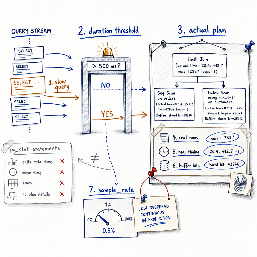
auto_explain changes that. It’s not a monitoring dashboard. It’s a crime-scene photographer built into the executor. When a query crosses a duration threshold, auto_explain writes the actual execution plan — with real row counts, real timing per node, real buffer hits — straight into the PostgreSQL log. No manual EXPLAIN ANALYZE, no app changes, no hoping the plan stays the same until you can reproduce it.

If you prefer watching, there’s a companion video that walks through the same diagnostic flow visually — the examples in this article match the ones shown there.

The problem: pg_stat_statements tells you “slow”, not “why”

pg_stat_statements is excellent at what it does: it normalizes SQL, then accumulates performance counters. You get calls, total_time, min_time, max_time, mean_time, stddev_time, shared_blks_hit, shared_blks_read, and more. It gives you a ranked list of queries by resource consumption. It’s the starting point.

But it records no plan shape. Not a single row estimate, not one node type. The plan that caused that max_time of 45 seconds? You’ll never see it from pg_stat_statements. You have to go hunting. You run EXPLAIN (ANALYZE, BUFFERS) manually, but the database is now under different pressure, the shared buffers are warm or cold, autovacuum may have run, physical reads differ. You get a plan that might resemble the one from the incident. You connect dots, but you lack the log line that proves it.

That’s the gap auto_explain fills — not by replacing pg_stat_statements, but by capturing execution-time detail that statistics aggregation throws away.

What auto_explain actually does

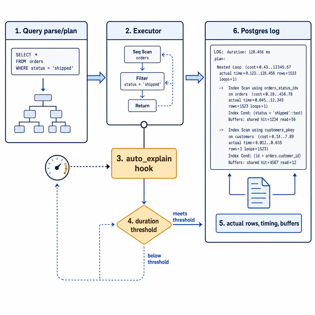
auto_explain is a contrib module bundled with PostgreSQL itself. It’s not a third-party extension; it ships in the contrib directory of every standard build. You don’t need CREATE EXTENSION. You load it at server start via shared_preload_libraries.

The module registers callbacks on the executor hooks ExecutorStart and ExecutorEnd. For every statement, the hook checks the elapsed duration after execution finishes. If that duration crosses auto_explain.log_min_duration (in milliseconds), the module calls ExplainQuery internally — the same EXPLAIN machinery you’d use manually — and writes the plan to the log. The flow looks like this:

                    +------------------------+
                    |  Query Optimizer       |
                    +-----------+------------+
                                |
                                v
                    +------------------------+
                    |  ExecutorStart         | <--- auto_explain installs hook, timer starts
                    +-----------+------------+
                                |
                                v
                    +------------------------+
                    |  ExecutorRun           | <--- Query executes
                    +-----------+------------+
                                |
                                v
                    +------------------------+
                    |  ExecutorEnd           | <--- duration checked, plan extracted if needed
                    +-----------+------------+
                                |
                 Duration > log_min_duration?
                                |
                       +--------+--------+
                       |                 |
                      YES                NO
                       |                 |
                       v                 v
            +--------------------+   +-------+
            | Write plan to log  |   | Close |
            +--------------------+   +-------+

If log_analyze is on, that plan includes the ANALYZE output: actual per-node timings, row counts, and loop counts. If log_buffers is on, you also get shared block hits and reads for each plan node.

Crucially, all this happens after the query completes. No instrumentation is injected before the threshold triggers. The timing overhead is incurred during execution only if log_analyze or log_timing are enabled, and the sampling knob sample_rate decides whether the plan is actually rendered and logged after the threshold is crossed.

Installing and enabling it

Check that auto_explain is available. On a self‑managed Linux install, the .so sits alongside other contrib libraries:

ls $(pg_config --pkglibdir)/auto_explain.so

If you installed PostgreSQL from packages, it’s almost certainly there. For managed services (Amazon RDS, Cloud SQL, Azure Database for PostgreSQL), it’s bundled in the engine image; you just need to enable it.

Add it to shared_preload_libraries in postgresql.conf:

shared_preload_libraries = 'auto_explain'

This requires a full server restart, not a reload. shared_preload_libraries is read once at server start because it determines which libraries the postmaster loads into every backend. A pg_ctl reload or SELECT pg_reload_conf() won’t change it. If you’re on a managed database, you update the parameter group / custom flags and then apply it — which typically triggers a restart (often during a maintenance window, so plan accordingly).

After restart, verify it’s loaded:

SHOW shared_preload_libraries;
-- should contain 'auto_explain'

Then you can set auto_explain.* parameters with a simple reload — they’re normal SIGHUP‑able GUCs once the library is loaded.

The core configuration knobs, one by one

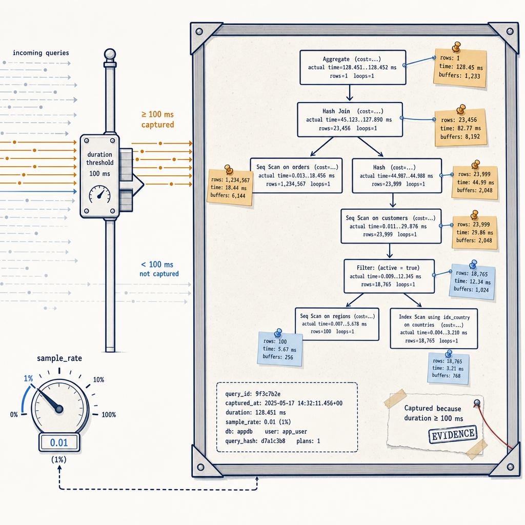
Here are all the relevant GUCs with their defaults and cost. Use this table as your reference.

| Parameter | Default | Description | Overhead | |-----------|---------|-------------|----------| | auto_explain.log_min_duration | -1 (disabled) | Threshold in ms above which a plan is logged. 0 logs every statement. | Minimal — only triggers after elapsed time, but if set to 0 you'll log every query, which can saturate disk. | | auto_explain.log_analyze | off | When on, the log includes actual per‑node execution time, row counts, and loops (EXPLAIN ANALYZE output). | Significant: adds per‑node instrumentation overhead, especially many clock calls. Use with sample_rate. | | auto_explain.log_buffers | off | When on, includes shared block hits, reads, dirtied, and written per plan node. Also local/dirty/temp info. | Low — just counts buffer access, but must be enabled with log_analyze to appear. | | auto_explain.log_timing | on (when log_analyze is on) | Enables per‑node timing. Disabling it removes node‑level times but reduces instrumentation overhead (no per‑node clock calls). | Turning log_timing off lowers overhead when log_analyze is on, at the cost of losing node‑level times. | | auto_explain.log_verbose | off | When on, includes output columns, schema‑qualified object names, and other verbose detail. | Low. | | auto_explain.log_settings | off | Logs modified planner parameters that affect the query (e.g., enable_seqscan). | Low. | | auto_explain.log_nested_statements | off | If on, logs plans for statements executed inside functions. Can flood logs with plans from procedural code loops. | Varies; usually best left off. | | auto_explain.log_triggers | off | Includes trigger execution statistics. | Low, but can produce voluminous output. | | auto_explain.log_format | text | text or json. JSON gives structured plan data for parsing with tools; text is human-readable. | JSON generation has trivial additional cost. | | auto_explain.sample_rate | 1.0 (always log) | Fraction (0.0–1.0) of qualifying queries that get logged. Applied after duration threshold is crossed, at statement level. | Essential overhead control: set to 0.1 and you only pay plan formatting/I/O for 10% of slow queries. |

The two knobs that matter most for overhead are log_analyze and sample_rate. log_analyze forces the executor to instrument every node, regardless of whether the plan is eventually logged. sample_rate decides which of those instrumented plans get serialized and flushed to the log. So you always pay the instrumentation cost when log_analyze = on, but you can dial down the I/O and plan rendering cost.

sample_rate: the overhead control knob

If you enable log_analyze, PostgreSQL adds node‑level instrumentation to every query that the hook sees. That means gettimeofday() or clock_gettime() calls at the start and end of each node, row counters, and buffer counters. On a high‑throughput OLTP system, this can add measurable CPU overhead. In extreme cases — a query that processes millions of rows through nested loops — the engine can call clock_gettime tens of millions of times, potentially doubling or tripling the execution time of that query. The overhead is cumulative across all queries, even those that run fast and never hit the logging threshold.

auto_explain.sample_rate does not reduce that per‑query instrumentation; it’s a stochastic gate afterward. When a query’s duration exceeds log_min_duration, the module rolls a random number. If it lands under sample_rate, the plan is written to the log; otherwise, it’s discarded. This ensures you still catch every kind of slow query — the sampling applies only to instances of the same normalised statement, so with enough executions you’ll eventually collect a plan for each problematic query pattern, just not every instance.

A safe starting point for production:

auto_explain.log_min_duration = 2000   # log queries >2 seconds
auto_explain.log_analyze = on
auto_explain.log_buffers = on
auto_explain.sample_rate = 0.1         # log only 10% of qualifying executions

Then watch the log volume and system CPU. If the overhead is manageable, tighten log_min_duration to 1000 or raise sample_rate to 0.25. If you’re logging too many plans and need to reduce disk I/O, drop the rate to 0.05. The key is to keep the evidence gathering continuous, not a one‑time debug session.

Reading real auto_explain output

Let’s walk through an annotated log excerpt. I’ve set my log_line_prefix so I can correlate lines:

log_line_prefix = '%t [%p]: [%l-1] '

With auto_explain.log_format = json, I can pipe logs into jq or any JSON‑aware log processor. But for readability, here’s a text‑format plan from a slow query caught in the wild.

2025-03-15 14:23:01.123 UTC [24789]: [v-1] LOG:  duration: 3203.456 ms  plan:
Query Text: SELECT * FROM orders WHERE status = $1;
Aggregate  (cost=1.25..1.26 rows=1 width=0) (actual time=3203.450..3203.450 rows=1 loops=1)
  ->  Seq Scan on orders  (cost=0.00..1.24 rows=50 width=0) (actual time=0.123..3203.400 rows=847293 loops=1)
        Filter: (status = 'backordered'::text)
        Rows Removed by Filter: 152707
        Buffers: shared hit=1204 read=18923 dirtied=0

That’s a crime scene in three lines.

• Row estimate vs actual: planner guessed `rows

=50, but the actual row count was 847,293 — a 16,000× underestimate. This alone explains why the planner chose a sequential scan, thinking only a handful of rows would match the filter. Without auto_explain, you'd never see the runtime row counts; you'd only have the cost estimates from EXPLAIN, which still assume 50 rows. The Buffers line shows 18,923 reads — evidence that the table wasn’t fully cached. Combined with the enormous row count, you can now make an informed decision: create an index on status, adjust statistics, or partition the table.

Diagnosing with confidence instead of guessing

Auto_explain turns anecdotal slowness into reproducible evidence. By capturing the exact plan (with real timings, row counts, and buffer I/O) at the moment of execution, you stop re-running queries under different conditions and hoping the plan reproduces. You can correlate plan changes with configuration tweaks, workload patterns, or data growth. Combined with pg_stat_statements for aggregate trends, auto_explain fills the critical missing piece. For teams managing large Postgres fleets, integrating logs with centralized monitoring can surface slow-plan patterns automatically. Tools like MyDBA can help you analyze and correlate these logs with query performance data, making the leap from reactive troubleshooting to proactive tuning. The next time your dashboard spikes, you won’t be guessing — you’ll have the crime scene photos.