Why Your Partitioned Tables Are Still Slow: A Deep Dive into PostgreSQL Partitio
Why Your Partitioned Tables Are Still Slow: A Deep Dive into PostgreSQL Partition Pruning
You spent your weekend slicing a massive, sluggish twelve-million-row orders table into one hundred monthly partitions. You write your first query against the new structure, expecting it to complete in milliseconds. Instead, the query takes nearly as long as it did before.
When you run EXPLAIN, you see a wall of text: a sequential scan on every single partition. The planner is scanning every partition in the table. That’s the gap partitioning promises to close, and pruning is the only bridge.
Why “I partitioned it” doesn’t mean “it’s fast”
Here’s a scene that repeats across every monitoring dashboard after someone deploys partitioning for the first time. Someone declares a range partition on order_date, one partition per month, one hundred partitions. The idea is that queries for a single day or month will touch only the relevant partition; the planner will prune the other 99 before the executor ever sees them.
Fast‑forward two weeks. A query that filters on order_date = '2024-02-15' still takes longer than expected. You grab the EXPLAIN output and see a Seq Scan on every partition — all one hundred of them. Not even a single Partitions removed line. The query is scanning 12 million rows when it should be scanning maybe 70,000.
If you want a visual walkthrough of the most common failure modes, the companion video “Postgres Partition Pruning: Why Your Queries Are Still Slow” covers them with EXPLAIN output you can reproduce. This article goes further: the exact planner mechanics, runnable SQL, and the edge cases that trip up even experienced teams.
Two flavors of pruning: planner‑time vs execution‑time
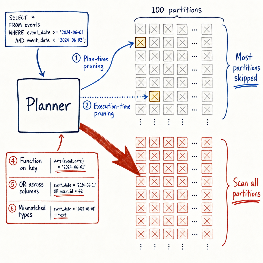
PostgreSQL prunes partitions in two distinct ways, and they show up differently in EXPLAIN. Confusing the two is the source of half the “but it’s still slow” reports.
Planner‑time pruning happens when the planner itself can see the literal value that restricts the partition key. The most obvious case is a hard‑coded constant in the WHERE clause:
SELECT * FROM orders WHERE order_date = '2024-02-15';If order_date is the partition key, the planner checks every partition’s CHECK constraints before execution and eliminates those that cannot possibly contain that date. The final plan only lists the surviving partitions — you won’t see the others at all. Planner‑time pruning has essentially zero runtime overhead; it’s just a tiny constraint‑exclusion check during planning.
Execution‑time pruning (also called run‑time pruning, available since PostgreSQL 11) kicks in when the value that determines the partition isn’t known at plan time. Common causes: prepared statement parameters ($1), variables inside a PL/pgSQL function, or values produced by a subquery. In these cases the planner cannot eliminate any partition during planning, so the plan text lists all partitions. But at execution, when the actual parameter value arrives, the executor evaluates each partition’s constraints and skips those that don’t match. You see the effect in EXPLAIN ANALYZE as a line like:
Subplans Removed: 97or, in newer versions:
Partitions removed: 97Execution‑time pruning still beats scanning all 100 partitions, but the overhead is higher. Each skipped partition still costs a few microseconds of constraint evaluation; for 99 skipped partitions the waste is negligible, but if you have thousands of partitions, those microseconds add up. And — crucially — execution‑time pruning falls back to planning‑time rules if the filter expression itself blocks constraint exclusion. Wrap the partition key in a function, and both flavors die.
Reading the actual EXPLAIN output — a worked example
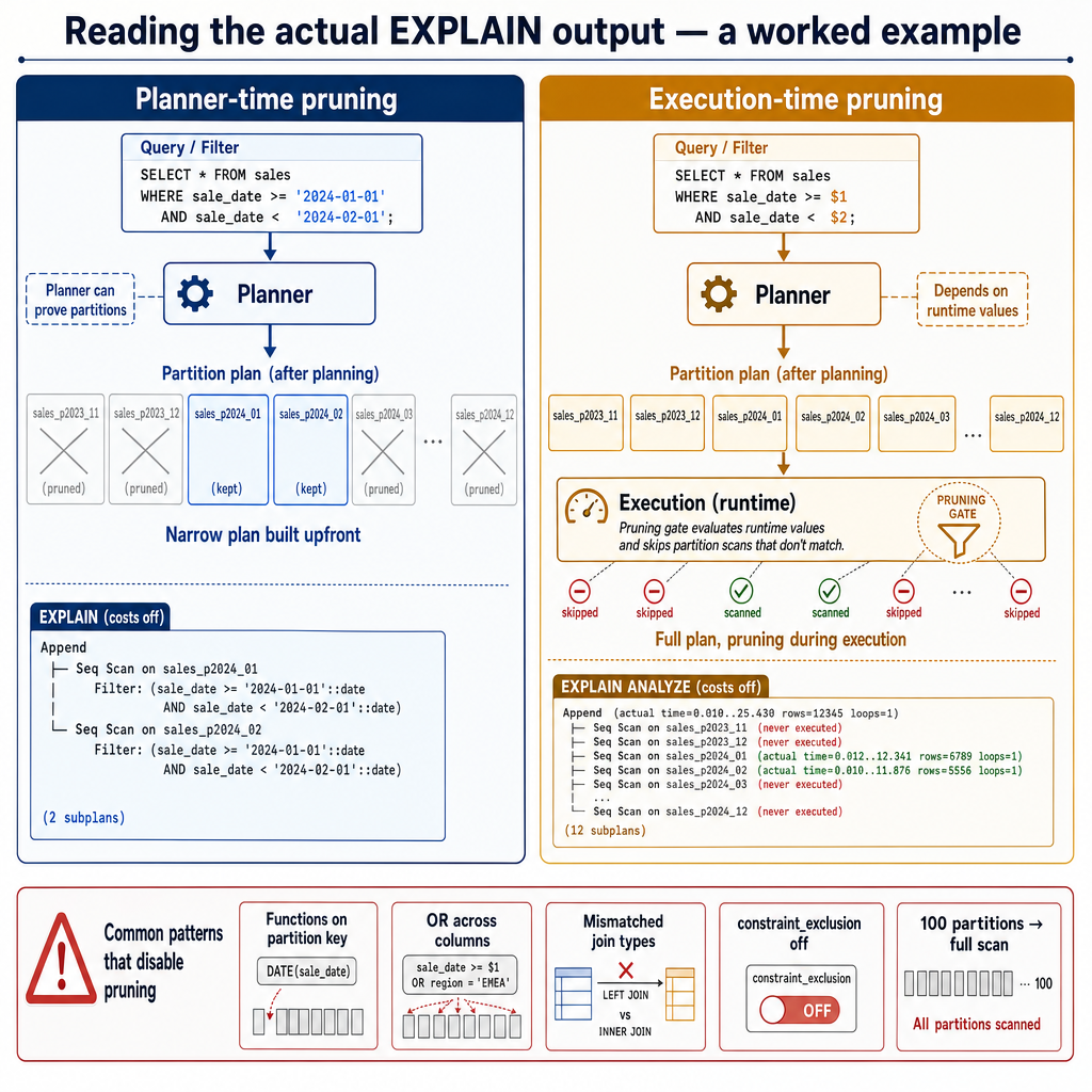
Let’s build a small partitioned table so you can run exactly this on your own instance. We’ll create an orders table with four monthly partitions.
CREATE TABLE orders (
    id bigint generated always as identity,
    order_date date not null,
    amount numeric
) PARTITION BY RANGE (order_date);

CREATE TABLE orders_2024_01 PARTITION OF orders
    FOR VALUES FROM ('2024-01-01') TO ('2024-02-01');
CREATE TABLE orders_2024_02 PARTITION OF orders
    FOR VALUES FROM ('2024-02-01') TO ('2024-03-01');
CREATE TABLE orders_2024_03 PARTITION OF orders
    FOR VALUES FROM ('2024-03-01') TO ('2024-04-01');
CREATE TABLE orders_2024_04 PARTITION OF orders
    FOR VALUES FROM ('2024-04-01') TO ('2024-05-01');

-- Insert a few hundred rows across all months so the table isn’t empty
Now query with a literal constant and inspect the plan:
EXPLAIN SELECT * FROM orders WHERE order_date = '2024-02-15'; QUERY PLAN
------------------------------------------------------
Seq Scan on orders_2024_02 orders (cost=0.00..28.00 rows=6 width=20)
Filter: (order_date = '2024-02-15'::date)
(2 rows)Only one partition appears. The planner eliminated the other three before the plan was assembled. That’s planner‑time pruning. You can measure the planning time by using EXPLAIN (ANALYZE, TIMING OFF, COSTS OFF), which keeps planning overhead but suppresses executor details; you’ll see a planning time of a fraction of a millisecond.
Now use a prepared statement, which forces execution‑time pruning:
PREPARE q1 (date) AS SELECT * FROM orders WHERE order_date = $1;
EXPLAIN EXECUTE q1('2024-02-15');
The plan lists all partitions:
                          QUERY PLAN
---------------------------------------------------------------
 Append  (cost=0.00..112.00 rows=24 width=20)
   Subplans Removed (at runtime): 3
   ->  Seq Scan on orders_2024_01 orders  (cost=0.00..28.00 rows=6 width=20)
         Filter: (order_date = $1)
   ->  Seq Scan on orders_2024_02 orders  (cost=0.00..28.00 rows=6 width=20)
         Filter: (order_date = $1)
   ->  Seq Scan on orders_2024_03 orders  (cost=0.00..28.00 rows=6 width=20)
         Filter: (order_date = $1)
   ->  Seq Scan on orders_2024_04 orders  (cost=0.00..28.00 rows=6 width=20)
         Filter: (order_date = $1)
(9 rows)
Notice Subplans Removed (at runtime): 3 — that’s the hint that pruning will happen at execution. But you can’t see which ones from the plan text alone.
Now run it with EXPLAIN ANALYZE:
EXPLAIN ANALYZE EXECUTE q1('2024-02-15'); QUERY PLAN
---------------------------------------------------------------------
Append (cost=0.00..112.00 rows=24 width=20) (actual time=0.014..0.015 rows=0 loops=1)
Subplans Removed: 3
-> Seq Scan on orders_2024_02 orders (cost=0.00..28.00 rows=6 width=20) (actual time=0.013..0.013 rows=0 loops=1)
Filter: (order_date = $1)
Rows Removed by Filter: ...
Planning Time: 0.120 ms
Execution Time: 0.045 msThis shows it: Subplans Removed: 3, and the only partition scanned is orders_2024_02. The planning time is higher than the literal case because the planner must still construct the full append structure, but the execution itself skips the irrelevant partitions.
WHERE‑clause shapes that enable pruning
For pruning to activate, the planner or executor must be able to map the filter condition directly onto a partition’s CHECK constraint. These patterns work reliably, provided the partition key column is used bare (no function) and the data types match the CHECK expression exactly.
- Equality on the partition key —
WHERE order_date = '2024-03-10'(range or list partition). - Range comparisons —
WHERE order_date >= '2024-03-01' AND order_date < '2024-04-01', includingBETWEEN. - IN lists on the key —
WHERE order_date IN ('2024-01-15', '2024-02-20')eliminates partitions for all months not referenced. - Hash partitioning — Pruning works the same way:
WHERE customer_id = 1024on a hash‑partitioned table, as long as the planner can compute the hash bucket from the constant.
List partitioning behaves similarly, matching against partition lists.
One subtlety: IS NULL and IS NOT NULL work if the partition definitions handle that. If your range partitions don’t include a default partition for NULL, a NULL search might scan all partitions. Declare a separate NULL partition or use a default partition if that’s the expected semantics.
The shapes that silently disable pruning (the real meat)
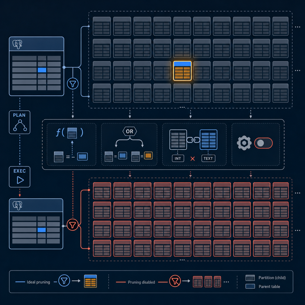
Here’s what you opened this article for. Each of these patterns will turn a precisely targeted partition query into a full‑scan across every partition. I’ve debugged each one at 2am. They rarely throw an error; they just burn CPU and disk.
1. Wrapping the partition key in a function
Any non‑sargable function applied to the partition key prevents the planner from matching it against the partition’s CHECK constraint. The most common culprits:
-- Bad: date_trunc, to_char, COALESCE, casting
SELECT * FROM orders WHERE date_trunc('month', order_date) = '2024-02-01';
SELECT * FROM orders WHERE order_id::text = '12345';
SELECT * FROM orders WHERE COALESCE(order_date, now()) = '2024-02-15';
All of these force a sequential scan of every partition. The fix is to move the function to the comparison side, or, if you need to truncate for a query pattern, consider an expression‑based partition key (supported since PostgreSQL 12):
-- Correct: avoid wrapping the key
SELECT * FROM orders WHERE order_date >= '2024-02-01' AND order_date < '2024-03-01';

-- Or create the partition by expression (if your access pattern always truncates):
CREATE TABLE orders_monthly PARTITION OF orders_partitioned_by_expr
    FOR VALUES FROM ('2024-02-01') TO ('2024-03-01');
-- with partition key: (date_trunc('month', order_date))
The rule is absolute: if the column is the partition key, the filter must reference the column directly, without any transformation, for pruning to survive.
2. OR conditions that involve non‑key columns
An OR on a non‑partition column, even when the other side of the OR targets the key, often defeats pruning. The planner sees a search that might require rows from partitions that satisfy the non‑key condition and gives up.
-- Bad: OR with a non-partition column
SELECT * FROM orders
WHERE order_date = '2024-02-15'
   OR amount > 5000;
The planner cannot prove that the amount condition won’t match rows outside the February partition, so it scans all partitions. The fix is to rewrite the query to use a UNION or UNION ALL to separate the conditions, allowing each branch to be pruned independently.
3. Joins with mismatched data types
When joining a partitioned table to another table, the prune relies on being able to compare the join condition against the partition’s constraints. A data type mismatch, such as joining a date column to a timestamp column without an explicit cast, can prevent the planner from implicitly mapping the values.
-- If orders.order_date is a date, joining on an apparent timestamp can fail
SELECT *
FROM orders
JOIN other_table ON orders.order_date = other_table.created_at;
-- If created_at is `timestamp with time zone`, pruning might not happen.
The fix is to use an explicit, correct cast or ensure the joined columns have identical types in the underlying schema.
4. Missing constraint_exclusion setting
For planner-time pruning to work, PostgreSQL needs to know that it should examine constraints. By default, constraint_exclusion is set to partition, which is sufficient for partitioned tables. If it has been changed to off (perhaps as a misguided optimization attempt), planner-time pruning will not occur. While execution-time pruning can still step in, the overhead increases. You should always ensure constraint_exclusion is partition (the default) or on.
SHOW constraint_exclusion;
-- Must return 'partition' or 'on'
Understanding these silent killers—functions, ORs, type mismatches, and configuration—is the difference between a lightning-fast partitioned query and a crawl of a hundred partitions. The EXPLAIN output never lies; if you see all partitions listed, one of these gremlins is almost certainly to blame.
Making Sure Pruning Survives in Production
Even after you’ve fixed the obvious killers, partitioned queries can regress. Schema drift sneaks in when someone changes a column type, new ORM-generated queries wrap keys in functions you’d never write yourself, and shifting data volumes turn a six‑partition scan into a hundred‑partition crawl. I keep a checklist taped to my mental desk: always run EXPLAIN on new query patterns, never let a function touch the partition key, rewrite ORs that span non‑key columns, and double‑check type alignment after every schema migration. If you’re managing hundreds of partitions across multiple services, that monitoring effort becomes a part‑time job—and missing one full scan can mean waking up to a pager at 2am.
Tools that automatically flag full‑partition scans save you from that phone call. MyDBA captures query plans from your production workload and highlights when pruning fails, so you catch the miss before it becomes a performance incident. No amount of careful partitioning replaces continuous observability, and no one should have to stare at EXPLAIN output all day. Keep your constraint mappings clean, watch for the silent killers, and let automation guard the bridge between your partitions and the planner.